An introduction to the 4 primary Prometheus metrics types

Prometheus is an open source metrics monitoring platform from the Cloud Native Computing Foundation. Its goal is to provide an easy starter UX and is designed as a single binary for ingestion, storage, and query. 

Prometheus monitoring has many widely adopted features and functionality, including its text exposition format, efficient metric store, and native query language called the Prometheus Query Language (PromQL). For stored Prometheus metrics, PromQL is the main way to query and retrieve the results you are looking for. 

There are four primary Prometheus metric types PromQL can query: counters, gauges, histograms, and summary metrics. These metric types fulfill the needs or requirements for most use cases, and are found in Prometheus’ official client libraries: Go, Java, Ruby, and Python. Note: each client library has its own documentation on how to use each metric type with the corresponding client library API. 

This blog explains Prometheus’ four primary metric types, covers when and how to use them, and gives resources for implementation.

Counter metrics are a fundamental way to track how often an event occurs within an application or service. They are used to track and measure Prometheus metrics with continually – or monotonically – increasing values which get exposed as time series. 

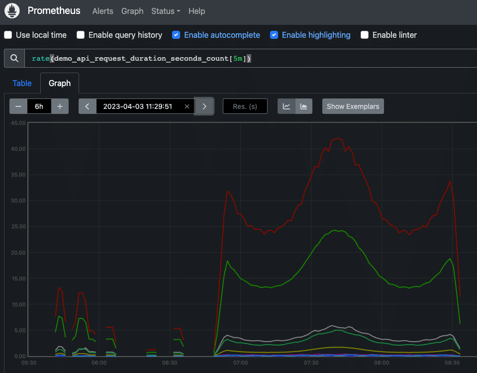
An example of a counter metric is http_requests_total, which reports the running total of HTTP requests to an endpoint on an application or service. The rate() function is applied to counters at query time in order to measure or calculate how many requests happen at a given time per second.  

Counter metricss are running or cumulative counts with metric client libraries that keep an ever-increasing total sum of the number of events for the lifetime of the application. These events can be periodically measured by having Prometheus scrape the metrics endpoint exposed by a client library. 

Running counts are highly reliable in that they allow for interpolation of any missed sample collections, which result in close approximations for an aggregation or total sum of values at a point in time. However, if you want to aggregate a running sum of many counts, you would need to apply a rate() function to visualize the changes per second on each count and then aggregate the counts with sum(). 

The below graph shows an example of a running or cumulative counter metric with the rate() function applied on a single count.

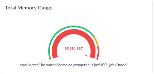
Gauge metrics are used to periodically take measurements or snapshots of a metric at a single point in time. A gauge is similar to a counter, however, their value can arbitrarily increase or decrease over time (e.g. CPU usage and temperature). 

Gauges metrics are useful for when you want to query a metric that can go up or down, but don’t need to know the rate of change. Note: the rate() function does not work with gauges as rates can only be applied to metrics that continually increase (i.e. counters). 

The image below shows an example of a gauge metric measuring memory usage over time in a dashboard component.

Histogram metrics sample observations by their frequency or count, and place the observed values in pre-defined buckets. If you don’t specify buckets, the Prometheus client library will use a set of default buckets (e.g. for the Go client library, it uses .005, .01, .025, .05, .1, .25, .5, 1, 2.5, 5, 10). These buckets are used to track the distribution of an attribute over a number of events (i.e. event latency). 

You can override these default buckets if you need more or different values, but note the potential increase in costs and/or cardinality when doing so — each bucket has a corresponding unique time series. 

Overall, histogram metrics are known to be highly performant as they only require a count per bucket, and can be accurately aggregated across time series and instances (provided they have the same buckets configured). This means that you can accurately aggregate histograms across multiple instances or regions without having to emit additional time series for aggregate views (unlike computed percentile values with summaries).

Prometheus client libraries support histogram metrics, allowing a service to record the distribution of a stream of data values into a set of ranged buckets. Histograms usually track latency measurements or response sizes. Prometheus histograms sample data on the client-side, meaning that they count observed values using a number of configurable buckets and expose buckets as individual counter time series.

Internally, Prometheus histograms are implemented as a group of counter time series that each represent the current count for a given bucket. The per-bucket counters are cumulative in Prometheus, meaning that buckets for larger ranges include the counts for all lower-ranged buckets as well. 

Each histogram bucket time series has an le label (“less than or equal”) and specifies the bucket’s upper value boundary as a number encoded in a string label value such as le=”0.05″ for an upper boundary of 0.05 seconds. Note that this adds an additional cardinality dimension to any existing labels that you track. 

This is what a Prometheus metrics histogram representation might look like:

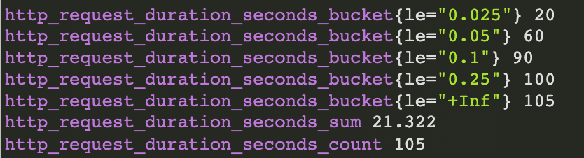
In this example, the first bucket is reporting 20, the second is reporting 60 (that’s 40 + previous 20), the third bucket is reporting 90 (that’s 10 + 60 + 20), and so on.

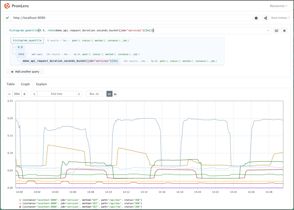
If you want to read your Prometheus histograms as percentiles or quantiles to better understand the distribution, then you would need to apply the histogram_quantile() function to estimate the requested quantile. 

This next graph shows a histogram as a quantile by applying the histogram_quantile() function to measure a demo service and calculate at what latency 90% of the API requests finish.

Summary metrics are similar to histogram metrics in that they track distributions of an attribute over a number of events, but they expose quantile values directly (i.e. on the client side at collection time vs. on the Prometheus monitoring service at query time). 

They are most commonly used for monitoring latencies (e.g. P50, P90, P99), and are best for use cases where an accurate latency value or sample is desired without configuration of histogram buckets. 

In general, summary metrics are not recommended for use cases where a histogram can be used instead. This is because quantiles cannot be aggregated, and it can be difficult to deduce what timeframe the quantiles cover. Note: this is defined by each client library independently (e.g. Prometheus Go client library uses 10 minutes by default).

Once client side quantiles are calculated, they cannot be merged with a quantile value from another instance. This means that summary metrics cannot be aggregated with any level of accuracy across time series. For example, the average of two P95 values does not equal the P95 for the combined set of values.

To learn more about how to implement each Prometheus metric type, refer to the documentation for the various Prometheus client libraries for Go, Java, Ruby, and Python. Prometheus also provides more in depth documentation. 

Let’s look at the four Prometheus metrics types and when to use them:

When tracking continually increasing counts of events you’d use a Counter metric. They are most often queried using the rate() function to view how often an event occurs over a given time period.

To report the current state of a metric that can arbitrarily increase or decrease over time, for example as a metric for CPU utilization.

These are showing the distribution of observations and putting those observations into pre-defined buckets. They are highly performant, and values can be accurately aggregated across both windows of time and across numerous time series. Note that both quantile and percentile calculations are done on the server side at query time.

Summary metrics measure latencies and are best used where an accurate latency value is desired without configuration of histogram buckets. They are limited as they cannot accurately perform aggregations or averages across quantiles and can be costly in terms of required resources. Calculations are done on the application or service client side at metric collection time. 

At Chronosphere, we provide a Prometheus-native and completely PromQL compatible metrics cloud monitoring solution along with optimized query and graphing functionality that works with the four primary Prometheus metric types.