Understanding cardinality over time in the real world

There is, however, another aspect of cardinality that was not previously addressed, and that is: how do you understand cardinality over time and at scale?

To enable our users to do just that, we built a new capability into the Chronosphere platform, the ability to analyze how cardinality changes over time with the cardinality_estimate() function. This builds on our Profiler capability that I covered in a recent blog, “Wrangle metric data explosions with Chronosphere Profiler.”

In today’s post, I’ll dive a bit deeper into:

• Why understanding cardinality over time and at scale is a difficult problem to tackle without the right tooling
• How Chronosphere Profiler and our new cardinality_estimate() query capability help with addressing cardinality over time
• Examples of the functionality in action

Tracking the cardinality of your time series data over time is extremely difficult. Unlike typical queries where you are usually interested in a subset of data in a particular service or application, cardinality is best understood at a broader level and over longer periods.

Use cases—such as determining which services have the highest metric churn, which metric names across all services are the most expensive, or which labels across your metrics have the most number of unique values—all require a more holistic view of your dataset. Standard open source tools don’t provide enough visibility, especially at scale. Instead, you need tools that provide an efficient way to query millions (or even billions) of time series as well as the ability to slice and dice your data over time.

Perhaps the best way to illustrate the complexity of this problem is an example…let’s suppose you have a service called `TheSignUpService` which, not surprisingly, handles the user sign-up flow for your application. `TheSignUpService` emits some rather critical metrics including `user_signup_duration_bucket` (a histogram tracking signup latency) with various labels, such as `status_code`, `city`, and, of course, `le`.

Business is going well, you’re expanding into different cities, and thousands of people are signing up daily. Over time, engineers working on this service improve the efficiency and, therefore, the buckets for this histogram (or `le`) become outdated. New ones are added so engineers can get a more accurate value for latency. However, as is often the case, this change is only additive, meaning the initial buckets continue to exist.

Fast forward six months,`TheSignUpService` dashboards are getting increasingly slow to load, graphs are timing out, alerts are failing to execute, and recording rules are showing gaps due to timeouts. Engineers need to pause their day-to-day work and figure out why this is happening.

Unless there is widespread query slowness across all services, the chances are good that high cardinality is the culprit. Unfortunately, to even see high cardinality, let alone act on it, you need to query all of the underlying time series. At this point, it is usually too late.

The good news is there are some steps you can take to start understanding current data cardinality:

1. If we take Prometheus-style metrics as an example, you can use the PromQL `count()` function to quantify the cardinality at a specific time (now or in the past). Here’s the issue we hit quite quickly: those queries must retrieve all the time series. When trying to do this at scale, you will eventually hit query rate limits or crash your time series database (TSDB).
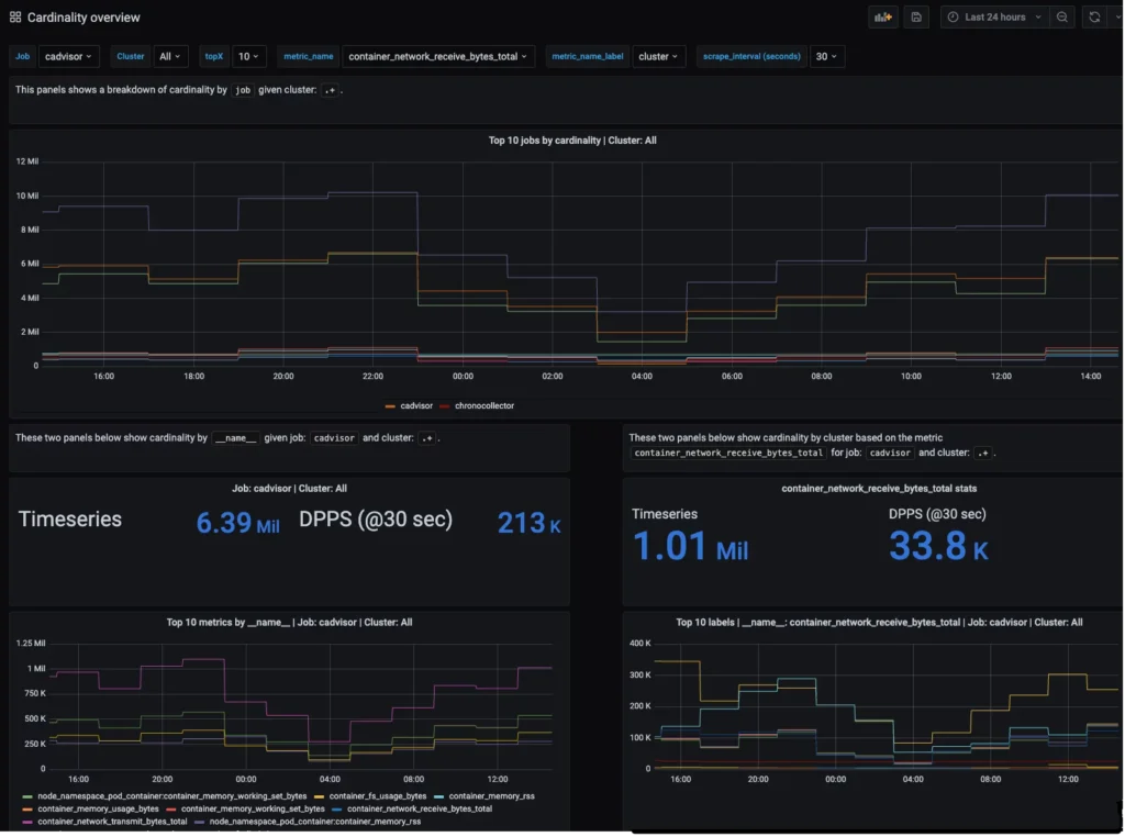
2. Chronosphere provides another extremely powerful way to inspect the data in real-time. It’s called the Chronosphere Profiler (read more about how it is used and its benefits). However, while Chronosphere Profiler gives you an unprecedented level of visibility of the live data as it’s being ingested, it will not be able to introspect historical data.
3. Most TSDBs track the overall number of time series managed over time, which can help you see if there is unexpected growth.

While these three approaches will get you part way to your goal of understanding cardinality over time, there are improvements that can make your life even easier from the perspective of:

• Applying to environments at a high scale
• Providing a historical view of the cardinality of the data
• Providing pinpoint accuracy of the source of increased cardinality

When you have extremely large data sets that are diverse and fluctuate over time, you need better tools. There will frequently be situations, especially when using microservices, where only a subset of the metric data is growing. When that happens, it becomes increasingly difficult to understand which subset of the metric data is growing and in what dimensions.

Making things more challenging: when fluctuations happen over time (e.g., due to scaling or changes in requirements—like the example with histogram sprawl above), it becomes near impossible to track and understand what was, and is, happening.

There are several frequently occurring cases with observability data increases that are extremely difficult to track down. Here are a few examples:

• A slow increase: This happens when the cardinality of a data set is notoriously difficult to understand. It is quite challenging to detect the change when comparing the current state against a day, a week, or a month ago.
• Data subset growth: how do you understand the difference between volumes of the same service from multiple deployments/AZ/regions or data centers? The overall increase may be easy to see, but delving into the how’s and why’s becomes hard to impossible.

The effects of these phenomena are reduced performance, increased cost, and effort to manage and leverage the data.

At Chronosphere, we have felt and heard about the pains and limitations posed by observability tooling in these areas for a while. That’s why we dedicate time to finding ways to make it easier to understand the extent of these situations for ourselves and our customers.

The data volume accounting features in Chronosphere and the Profiler are a great first step. With the addition of cardinality_estimate() to the Chronosphere platform we now provide a way to get an approximate cardinality for an arbitrary set of time series at any point in time.

Cardinality_estimate() supports a custom PromQL function that enables you to query and graph the cardinality of the metric data. We enable the user to specify filter(s) and return the cardinality of the time series matching the criteria, now and in the past (for however long the retention policy of the data is).

To understand better how cardinality_estimate() works, let’s try to compare it with the alternative count() function:

• Data in Chronosphere’s data store is organized into blocks for a given namespace.
• A block is defined by its size and could be any value representing the duration of time (let’s say 2h).
• So the number of series which needs to be read increases dramatically when longer queries are executed.
• All these fetched time series would be loaded in DbNode’s memory and then transferred to read coordinators.
• Because of this huge overhead, count() queries, issued for longer time intervals and containing millions of time series data, would almost always fail because resource usage is too high (providing there is a level of separation built into the TSDB used, otherwise it might crash the node).
• For the simple count() function, the Prometheus query engine will need to read all the time series for each block, satisfying the given query and then aggregate the results by simply incrementing the counter.
• If the query is issued for the last 24 hours, the query engine needs to read at least 12 latest blocks to fully collect all data.

The cardinality_estimate() function takes a completely different approach that greatly reduces cardinality (and therefore won’t crash the node). Since we’ve implemented this custom function from scratch, we were able to use internal database data structures to our advantage. Here’s how it works:

• When each query is executed, the reverse index is used to find the actual data. This satisfies the given query quickly. (We won’t dig deeply into how the reverse index works now, but we’ll just mention that it uses roaring bitmaps – which can be best described as better compressed bitsets.)
• Queries support fast and efficient operations on sets, like intersections, unions, etc. The result of query execution is typically an iterator, which means iterating the query results and doing some operations/aggregations on top.
• With cardinality_estimate() we can actually do better. Because we know that we are only interested in the cardinality of our results—instead of iterating and decoding data points through all the resultset—we can just use the cardinality value from the roaring bitmap of an already executed query.
• All these cardinality values are already computed and returned from the data store nodes to the read coordinators, so the amount of data we need to transfer over the wire is heavily reduced.
• Since the roaring bitmap is stored once per block, our data resolution becomes the same as the block size. This means that we lose some data granularity compared to count(). However, we can execute fast cardinality queries over large intervals of time with arbitrary filters applied. This narrows the scope to data subsets and potentially covers millions of different time series.

There are several failure patterns encountered “in the wild” when dealing with metric data where cardinality_estimate() can be invaluable. Here are a few common examples:

• In a microservices (and even a monolith) architecture, adding new application capabilities can cause a slow (or not so slow) increase of observability data.
• Large impacts of mistakes and anti-patterns in the service instrumentation cause cardinality growth. For example, labeling metric data with unique identifiers is common.
• Scaling up the infrastructure or replication factors of services and components has a huge impact on cardinality growth. In those instances, if you track 100 time series for a container, and the number of containers goes up 50%, so will your data volume with various consequences described in our problem statement in the beginning. The situation is exacerbated when this happens frequently and in a short time span. The increase in active time series caused by this churn can be quite serious.

With the capabilities Chronosphere provides, users can immediately start dissecting the data set when these situations occur. The game-changing difference: You can understand the volume/cardinality and the context of a specific time series.

For example: 

sum(rate(http_response_code{service=’login`, geo=`apac`})) by (country, respcode) will give you the raw response codes per country and respcode, and you can infer that it increased for a certain country, but it doesn’t tell you by “how much.” You are missing a last known good baseline and the scale of the change.

In contrast, cardinality_estimate() allows you to run the following query, providing the cardinality of a subset of data now and over time.

cardinality_estimate(http_response_code{service=’login`, geo=`apac`, country=`australia`})

This means you can compare the baseline with the current state, and specifically drill down on a per-label value based on how much it changed.

Best of all, you can build cardinality_estimate() into alerts and dashboards to enable your broader team to self-service – when double checking the effects of a deployment or understanding the magnitude and source of a potential issue.

Generally, when fluctuations in data occur, a fast response is essential since the impact can be quite severe. It would not be surprising that a user or administrator of an observability tool would detect and analyze an event of this type using the capabilities described in the previous section.

After understanding the problem, it needs to be acted upon. Depending on the situation, your responses may vary. You can control the data on the generation side (if we’re not talking about scaling – i.e. if an organization is scaling up infrastructure due to an increase of paying customers, you probably don’t want to pump the breaks on it).

The control plane of the Chronosphere platform was purpose-built just for that and enables you to act upon a situation of this type rapidly. Here’s how:

• Alert on the occurrence of cardinality growth
• Provide the ability to drop less valuable subsets of data and not cause a loss in visibility
• Aggregate – In the long term, you can put Chronosphere control plane rules in place that will reduce the cardinality of metrics of your choice, to maintain sufficient visibility, performance, and keep the volume in check.
• Keep track of cardinality sources and confirm instrumentation best practices are followed across the organization.

Leveraging these capabilities gives you an unprecedented instant way to:

• Proactively control the volume and cardinality of the data you manage and get alerted when defined boundaries have been over-stepped.
• Understand the shape and volume of data using volume accounting, profiler, and cardinality_estimate to identify the root of the change.
• Control the volume using drop policies and roll-up rules to avoid potential cost and performance implications.

Introducing oversight and predictability in your observability tooling gives the control back to the users and administrators, ensuring predictable performance, cost and reliability.