Using aggregation rules to control data growth

At Chronosphere, we believe in giving teams the control over observability data that they need to ensure that they get the value they expect, without paying unnecessary costs. One of the essential tools that we provide to do this is aggregation rules. Aggregation rules allow our customers to send us high-cardinality, high-resolution metric data, and then rollup or downsample metrics as they see fit before they are stored – this gives clients broad flexibility to reduce the cardinality/volume of their metrics in ways that other solutions simply cannot. Today we’ll walk through three examples of how you can use aggregation rules, based on some of the use cases we’ve seen with our customers.

This is probably the most common example of how we see aggregation rules used since it applies to most organizations that have adopted cloud-native architectures. Suppose you have a stateless microservice, that is configured to autoscale based on the incoming traffic your service needs to handle – there might be just a handful of containers during low traffic periods, but at peak, you could have dozens, even hundreds of instances running to support user demands. These containers will almost certainly emit metrics on their behavior that we want to collect to understand how healthy the service is overall. But do you actually look at these metrics on a per-instance basis? It’s doubtful – we usually care about things like request latency at the overall service health, not a single replaceable container out of many.

Let’s take some real numbers using a metric for how many requests a hypothetical service is handling:

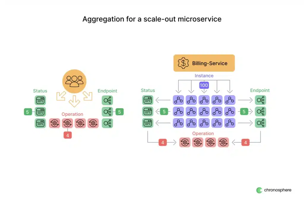
n the above, we assume our billing-service is running across 100 containers emitting metrics, each reporting on total requests across 5 separate endpoints, with 4 possible operations, and 5 potential status codes. For example, an individual timeseries reported by a container might look like this:

http_requests_total{service=”billing-service”, endpoint=”/bill”, operation=”GET”, status= “200”}

In reality, we probably want to have additional labels such as region, cluster, and so on, but we’ll keep it simple for now. If we look at the total cardinality of the metric based on the above labels, we can see that there will be 100 * 5 * 5 * 4 = 10,000 unique time series that we are tracking. Since we’re not interested in looking at this metric on a per-instance basis though, we can create an aggregation rule to roll it up before we store it.

As a result of such a rule, the cardinality added by the instance label can be eliminated, which in our example will reduce the number of unique time series to just 100. That’s a 99% reduction! Additionally, with Aggregation Rules, it’s easy to generalize them to apply to all of the counter metrics our billing-service emits, and not just our http_requests_total metric. That means that if we add additional metrics, we don’t have to worry about adding more rules, either. Pretty neat, right?

Our first example shows the power and simplicity of aggregation rules, but there are a lot more ways we can use them to control our metric data. Let’s take a look at another example that deals with metrics from a service we don’t control.

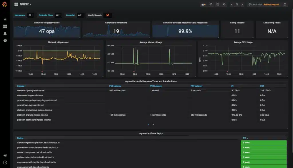
There are a lot of off-the-shelf applications that can emit Prometheus metrics natively, and do quite a good job of providing visibility into the work that they do. Ingress controllers such as nginx or istio are excellent examples; they give us pretty extensive metrics on their behavior, and usually come with community-built dashboards to help us get quick visibility into how they are operating.

Depending on your use-case, the metrics that an ingress controller like nginx emits may be higher cardinality than you need. Alternatively, you may take advantage of all of the labels that are available for its metrics, but not all at once – for example, looking at request traffic based on ingress vs looking at it by namespace. Let’s look at a concrete example of what we can do here with aggregation rules to control cardinality in this kind of situation:

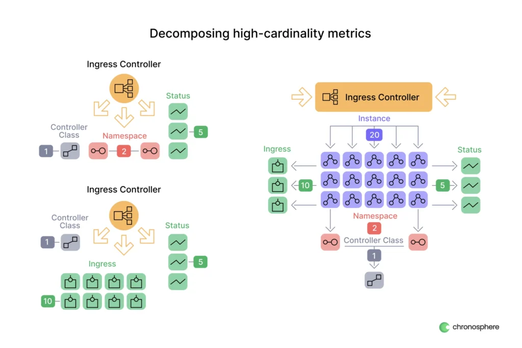
This is a pretty simple example, but if we look at the combined cardinality of the labels we have  20*10*5*2 = 2,000 unique timeseries. It’s clear how quickly this will grow as the size of our cluster and the complexity of our ingress rules will grow. We can reduce the overhead though, by using aggregation rules to create two new metrics, one for the per-ingress and one for the per-namespace case.

In a case such as this, we can define two rules, with each one retaining the explicit set of labels we want to keep, and omitting the ones we do not use. If we look at the cardinality of our two aggregated metrics we have a total of:

20*5*10 + 20*5*2 = 1,200 unique timeseries

Not bad, almost a 50% reduction just by that simple breakdown. If we don’t need the instance label like in the first case, then it gets even better – we’d drop to just 60 unique time series!

This example shows how we can decompose highly dimensional, high-cardinality data before we store it to cut down on the amount of data we need to keep overall. Remember, additional dimensions and cardinality are multiplicative, but by splitting a metric with several dimensions into multiple metrics with fewer dimensions, we can reduce the total amount of data, essentially factoring out dimensions that would otherwise be multiplied together.

Let’s go back to the first example we looked at with a scale-out microservice. Our original set of labels was pretty simple, but sometimes we want to add additional dimensions to give us granular insight into the user experience. For example, what if we wanted to add a dimension to our billing-service metrics that identified the customer that was being served? That’s going to increase our number of time series by a significant amount, even if we have a relatively small number of customers:

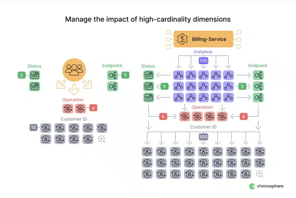
n the example here, we have just 300 unique values for customerID, but that brings our total number of time series to 100*5*5*4*300 = 3 Million! Even with our original aggregation rule to remove the instance label, we’ll still be looking at 30,000 unique series, which is not a small number. The more services we add this label to, the more growth we’ll see. Not only that, we should assume our list of customers will grow as well.

So what can we do here? Well, what if we don’t actually need this granularity for all of our customers? We could potentially limit it to a smaller cohort, say the top 10 biggest clients that we serve. This could be done by maintaining a list of customers to emit the per-customerID label for, but we can also keep the logic separate from the application using aggregation rules.

In a scenario like this, our aggregations would be similar to what we’ve described in the cases above – we can create one rule that eliminates both the customerID and instance labels, and a second rule that just eliminates the instance label, but is scoped to only match the set of customerIDs we are interested in retaining. This way, we can get granular insights for our top 10 clients, without having to store the cardinality for all of our other clients. Even better, if we need to update the list, it’s a simple change to the rule, no code changes are needed! What about the impact on cardinality though?

5*5*4*10 + 5*5*4 = 1,100 unique timeseries

We’ve gone from 3 Million to just 1,100 – that’s a 99.96% reduction in cardinality.

We’ve gone through just a few of the real use cases we’ve seen where aggregation rules have helped our customers manage the growth of their metric data. There are plenty of more specific scenarios where aggregation rules can be applied to reduce costs or improve performance as data scales, but hopefully, the examples we covered have given you an idea of the possibilities here. If any of these seems like they would apply to your data, or if you’re struggling with out-of-control metric growth, let us know! We’d love to hear from you and discuss how Chronosphere can help.